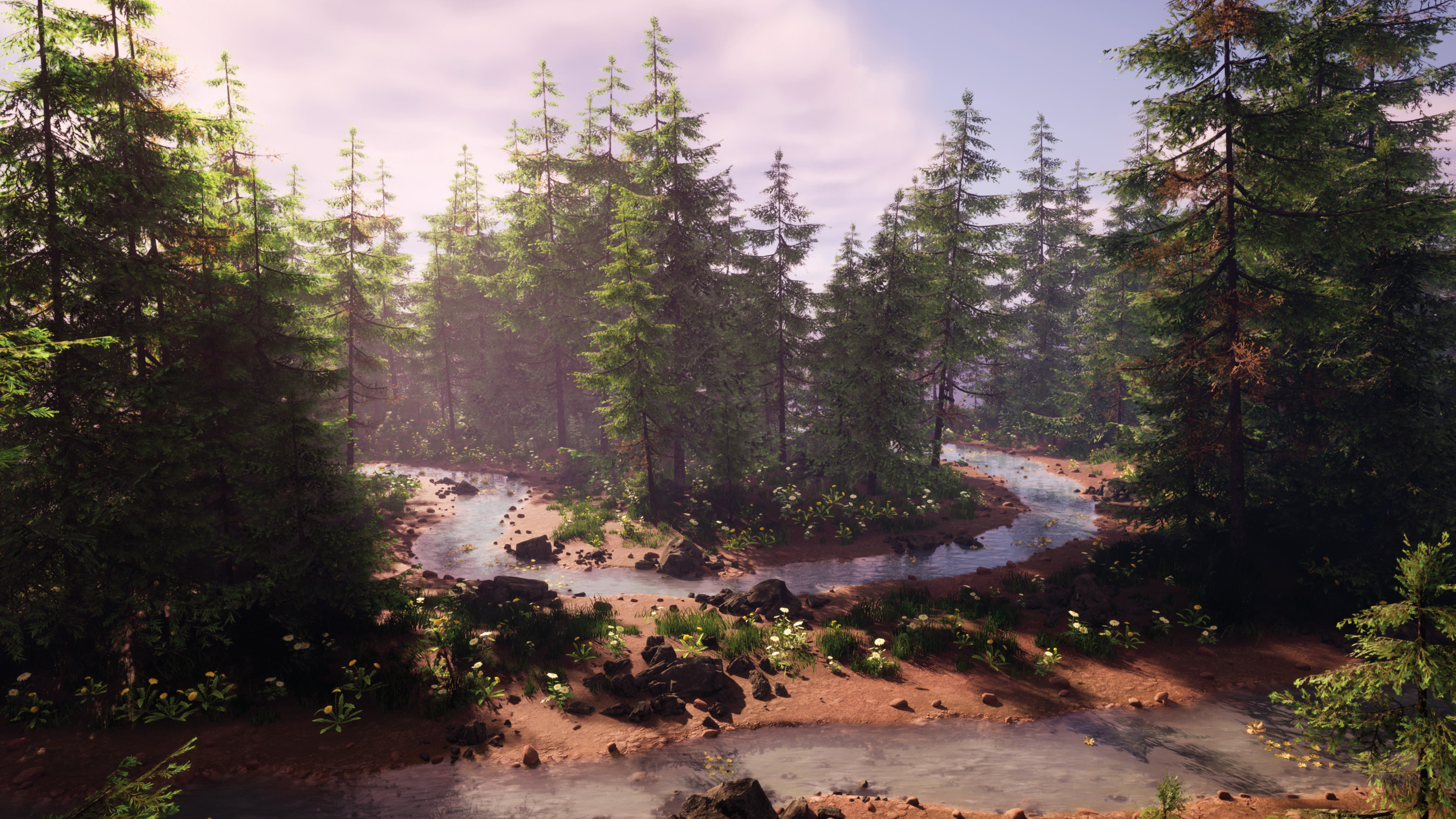
Procedural modelling has been on the rise in recent years, with Houdini leading the charge as the go-to software for proceduralism and VFX. But other 3D content creation tools are catching up and offering their own solutions. During this year’s Game Developers Conference, Epic Games unveiled its new in-house tool, Procedural Content Generation (PCG), within Unreal Engine 5, sparking discussions and inspiring new creative works.
PCG empowers artists to establish rules for generating environments procedurally in the Unreal Editor, allowing for real-time adjustments. Despite still being in its early stages, PCG presents a compelling alternative to Houdini and Houdini Digital Assets due to its integration and elimination of the need for additional software.
The tools show performance advantages, using a node-based workflow similar to Houdini. This grants access to point data and enables custom attribute creation and manipulation, as well as randomisation and scattering.
It’s important to note the current version is mainly focused on instantiating assets rather than creating them from scratch. However, Unreal Engine does offer other facilities to model geometries procedurally. For more information take a look at Creative Bloq's guide to Unreal Engine: everything you need to know, as well as the Unreal Engine 5 review.
Making an environment in UE5: the process
For this tutorial, readers are expected to know the basics of Unreal Engine 5 and the Blueprint Editor. Knowledge of Houdini can be helpful, but isn’t required.
01. Preparing the testing assets
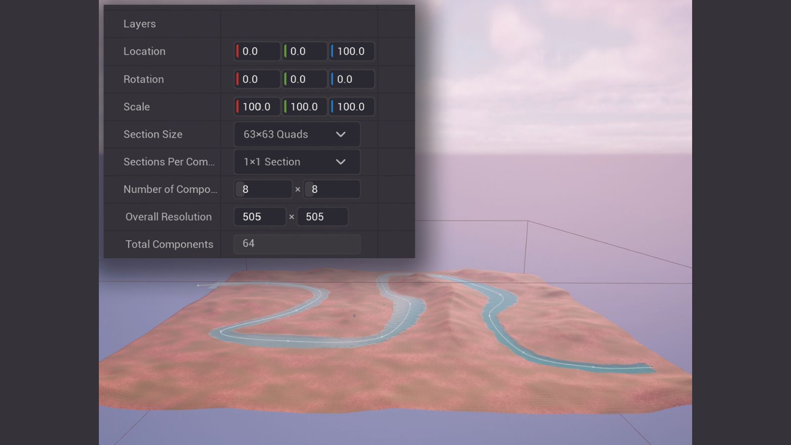
A landscape is needed as the starting point of our project, it’s advised to create a small enough landscape from a new basic level instead of the default large open-world level. A river is also added to allow the population of different assets in the river area. The shape of the landscape is applied with a simple noise brush.
I’d encourage you to spend more time refining its shape or get the Heightmap generated with third-party software. We’ll start scattering points to instantiate the trees on the landscape next.
02. Understanding basic scatterings
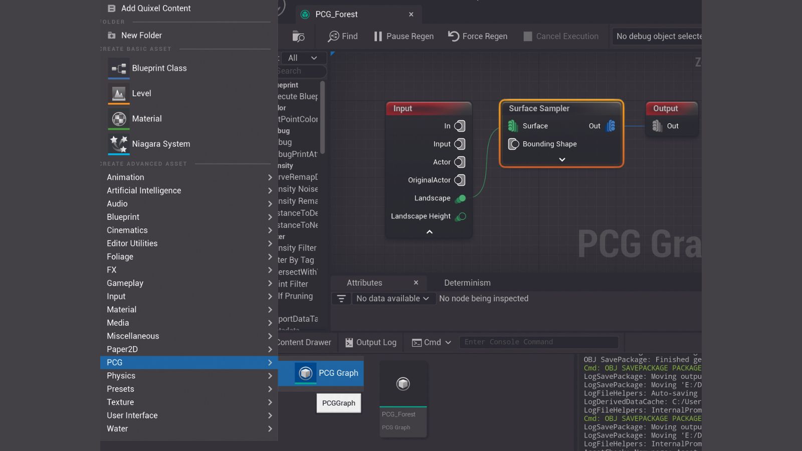
Create a folder called ‘PCG/PCG_Forest’ in the Content Browser, right-click, and select PCG>PCG Graph. Name the newly created graph ‘PCG_Forest’ and open it. The central area of the window with the Input and Output nodes is the graph that will form the basis of our procedural rules.
Right-click on an empty area, search for Surface Sampler and hit Enter to create it; a process that works for creating any node. Expand the Input node, drag the Landscape output pin, and drop it to the Surface input pin of the Surface Sampler node to connect them. Connect the Out output of the Surface Sampler node to the Out input of the Output node.
03. Run a scattering test
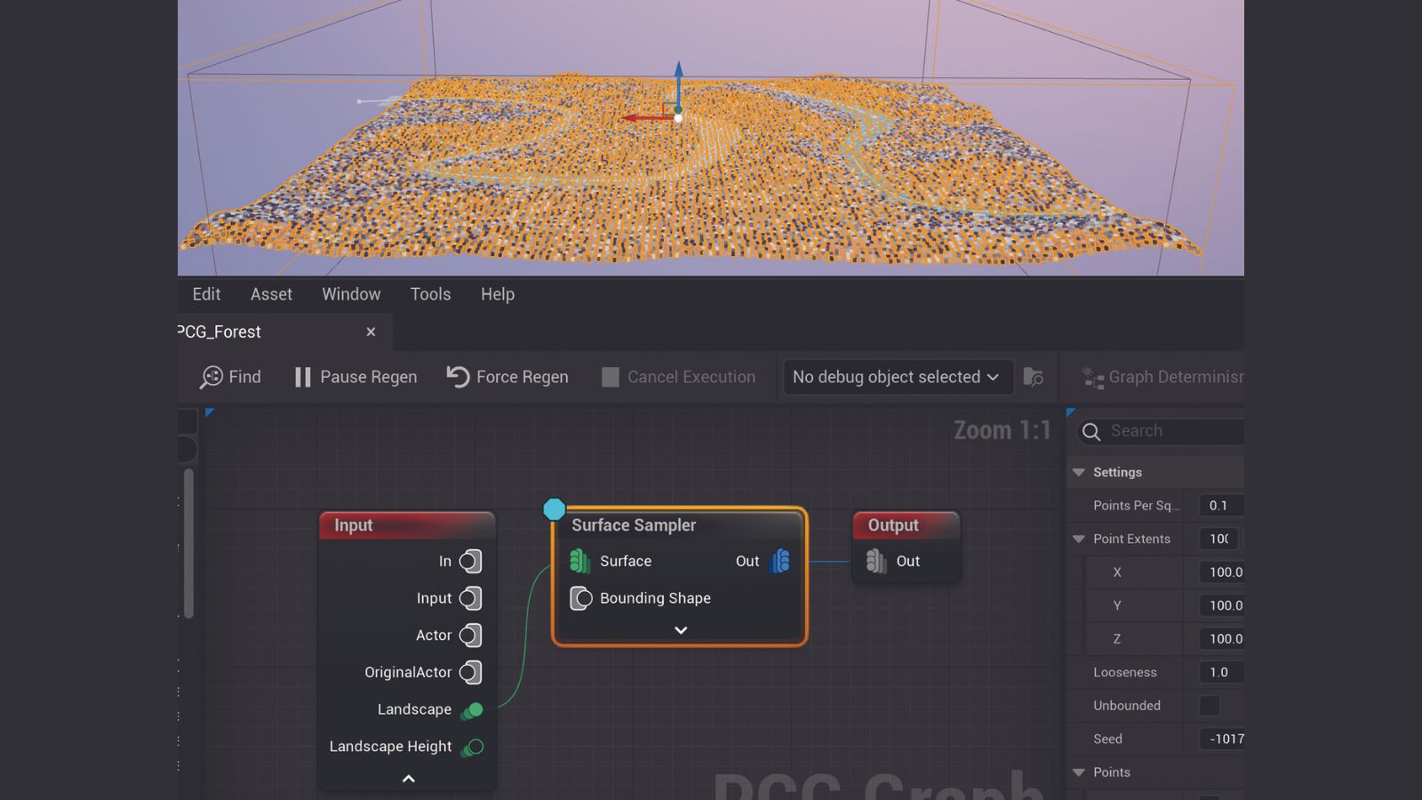
Drag PCG_Forest to the centre of the world, and scale so its bound covers the entire landscape. Select the Surface Sampler node and press ‘D’ to toggle on its debugging. A massive number of points in greyscale colours should appear on the landscape.
The Surface Sampler samples the landscapes and scatter points on it. Each point holds Location, Rotation, Scale, Density, and many other attributes. Their colour resembles the value of the Density attribute, with brighter meaning a bigger Density value. We’ll eventually instantiate tree meshes on these points. Press ‘D’ again to toggle debugging off.
04. Remapping density by height
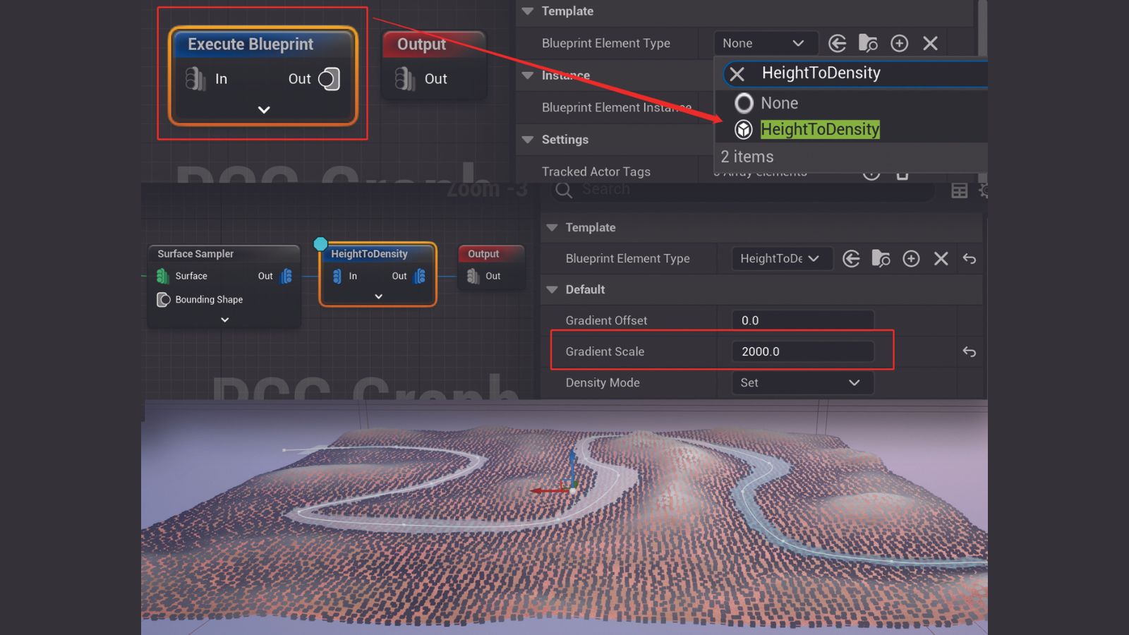
Disconnect the connection between the Surface Sampler and Output nodes by Alt-clicking any of its pins. Create an Execute Blueprint node and set its Blueprint Element Type to HeightToDensity. Connect the Out output of the Surface Sampler to the In input of the HeightToDensity node, and connect the Out output of the HeightToDensity node to the Out input of the Output node.
We’ve basically inserted a HeightToDensity node between the Surface Sampler and Output nodes. Set the Gradient Scale of the HeightToDensity node to 2000, and press ‘D’ to toggle debugging. You should see the colour of the points get brighter when their position is higher.
05. Calculating the height range
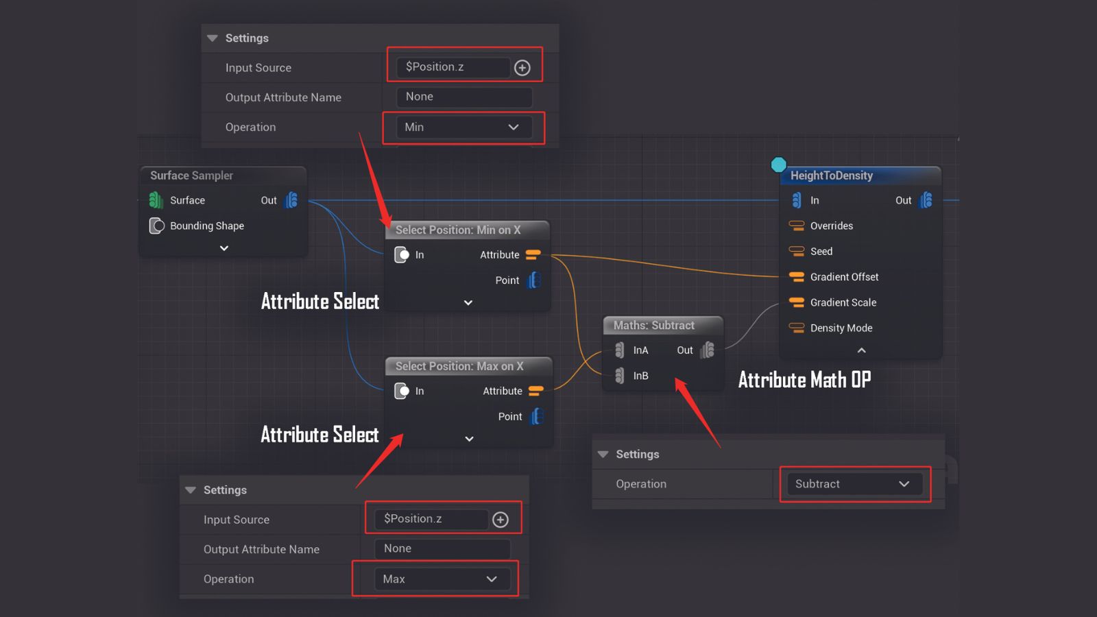
Create a pair of Attribute Select nodes and an Attribute Math OP node, and then connect them between the Surface Sampler and HeightToDensity node as shown. For the Attribute Select node on the top, the Input Source is set to $Position.z, which means it reads the Z value (vertical) of the Position attribute of the points.
Set the Operation to Min so that we’re reading the minimum Z position of all points in the Surface Sampler. For the bottom Attribute Select node, we set the same Input Source with the Operation set to Max. The Operation of the Attribute Math OP node is set to Subtract. We’re simply saying that from the lowest point to the highest point, remap their Density from 0 to 1.
06. Filtering the points
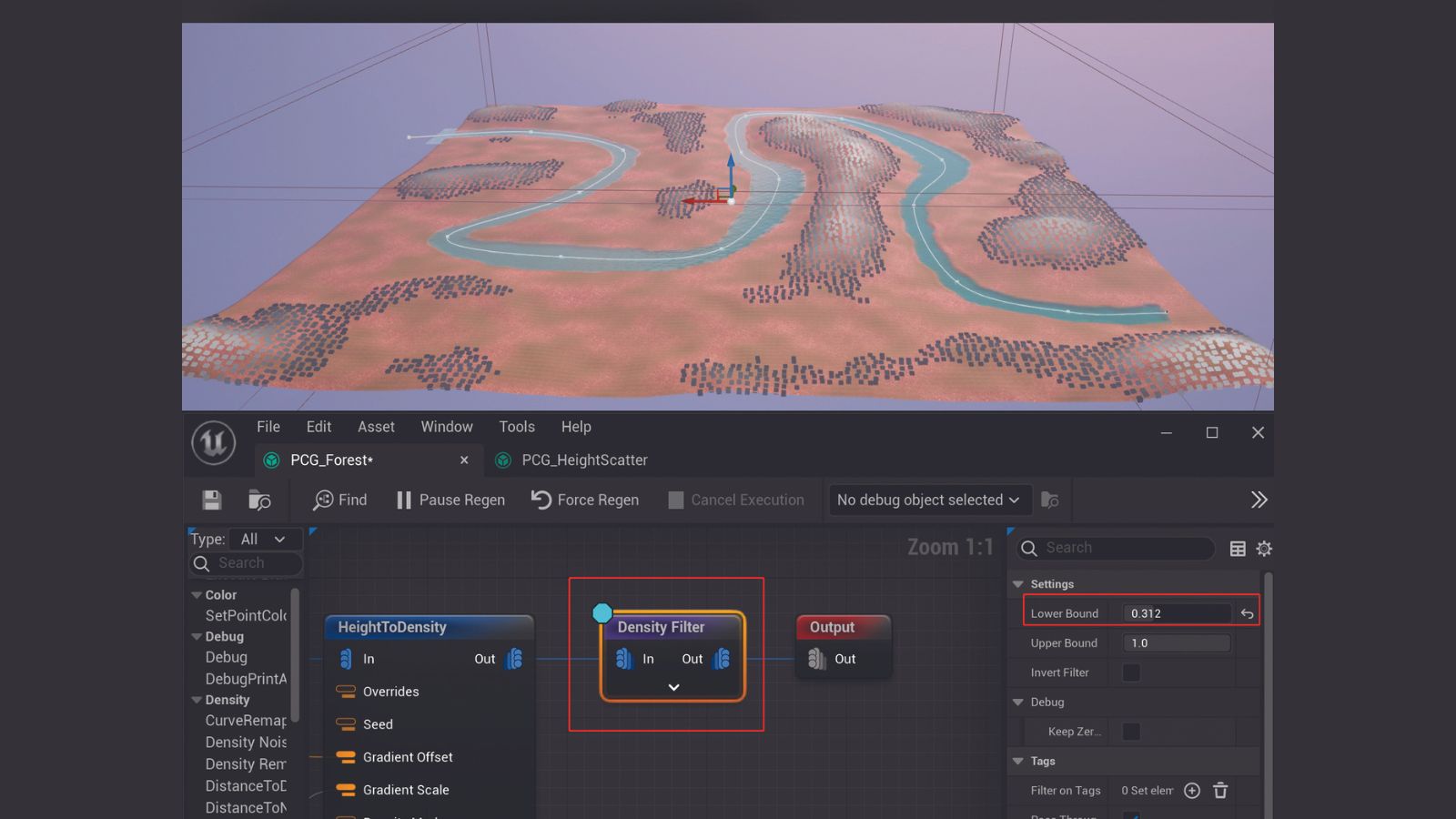
Insert a Density Filter node between the HeightToDensity and Output nodes. Set its Lower Bound to 0.312, and Upper Bound to 1.0. Any points with a density value outside of the 0.312-1.0 range are now filtered out, leaving only the points on the high ground visible. Disable the debugging for the HeightToDensity node and enable debugging for the Density Filter to see the effect.
07. Randomly filter out more points
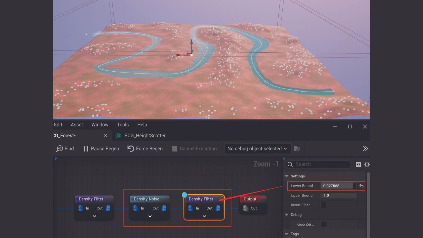
Insert a Density Noise and another Density Filter node between the previous Density Filter and Output nodes. Set the Lower Bound of the new Density Filter node to 0.9 and we should see far fewer points left on the high grounds.
The Density Noise node will randomise the Density attributes of the points and the Density Filter filters out the points based on their Density value. This is a typical way of randomly removing points.
08. Insterting trees
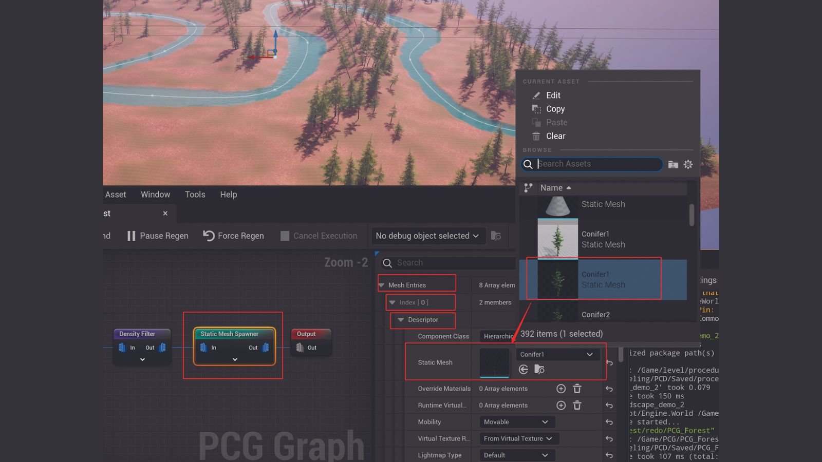
Have a few tree models ready and waiting to go. A natural environment pack including trees, rocks and other foliage is now added to the project. Create a Static Mesh Spawner node and insert it between the Density Filter and the Output node. Open the Mesh Entries attribute and add a few entries by pressing ‘+’.
Now open the Descriptor section in each of the entries and set the Static Mesh attribute to a different tree. The trees should now be randomly inserted at each point generated in the previous step.
09. Adding tree transform variations
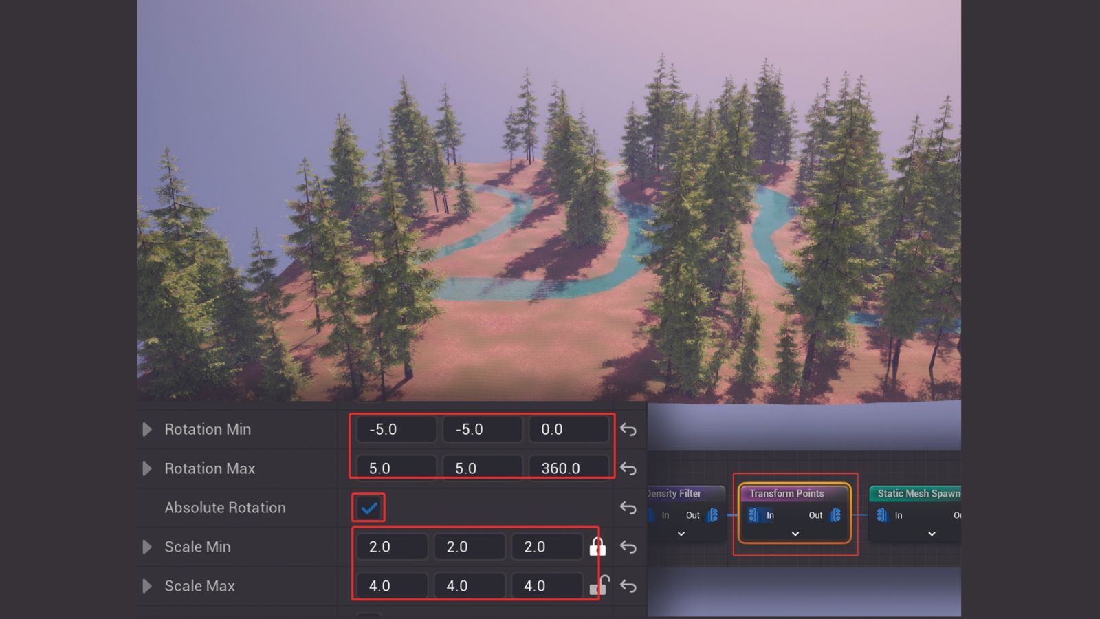
Insert a Transform Points node between the Density Filter and Static Mesh Spawner nodes. Set the Rotation Min values to -5, -5, 0 and Rotation Max to 5, 5, 360, which makes the trees randomly rotate on the X, Y, and Z axes. To avoid trees following the slope of the landscape surface, check the box for Absolute Rotation. Set the Scale Min and Scale Max to adjust the overall size and size variations.
10. Creating points around trees
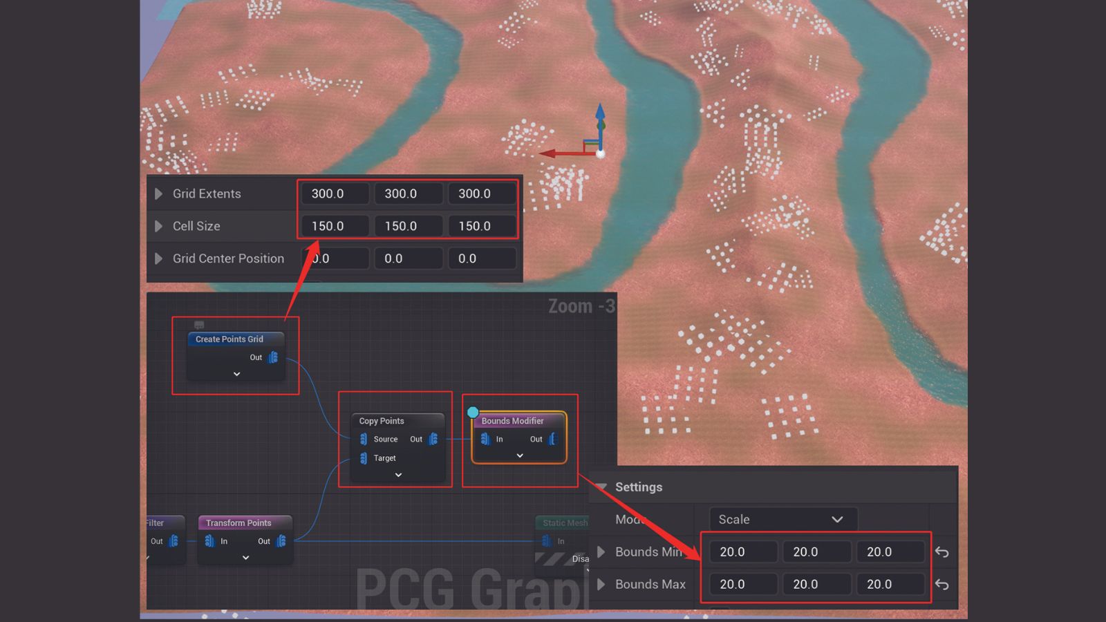
Select the Static Mesh Spawner and press ‘E’ to disable it. Make a new Create Points Grid node, and Set its Grid Extents values to 300, and Cell Size to 150, making a simple 600x600 point grid with each point 150 units apart.
Create a Copy Points node, connect the output of the Create Points Grid node to its Source input, and connect the Transform Points node to its Target input. The Copy Points now copies the point grid to each point of the Transform Points node. To visualise the points, create a Bounds Modifier node, connect the output of the Copy Points node to its input, set the Bounds Min and Bounds Max values to 20, and toggle on its debugging.
11. Randomising points around trees
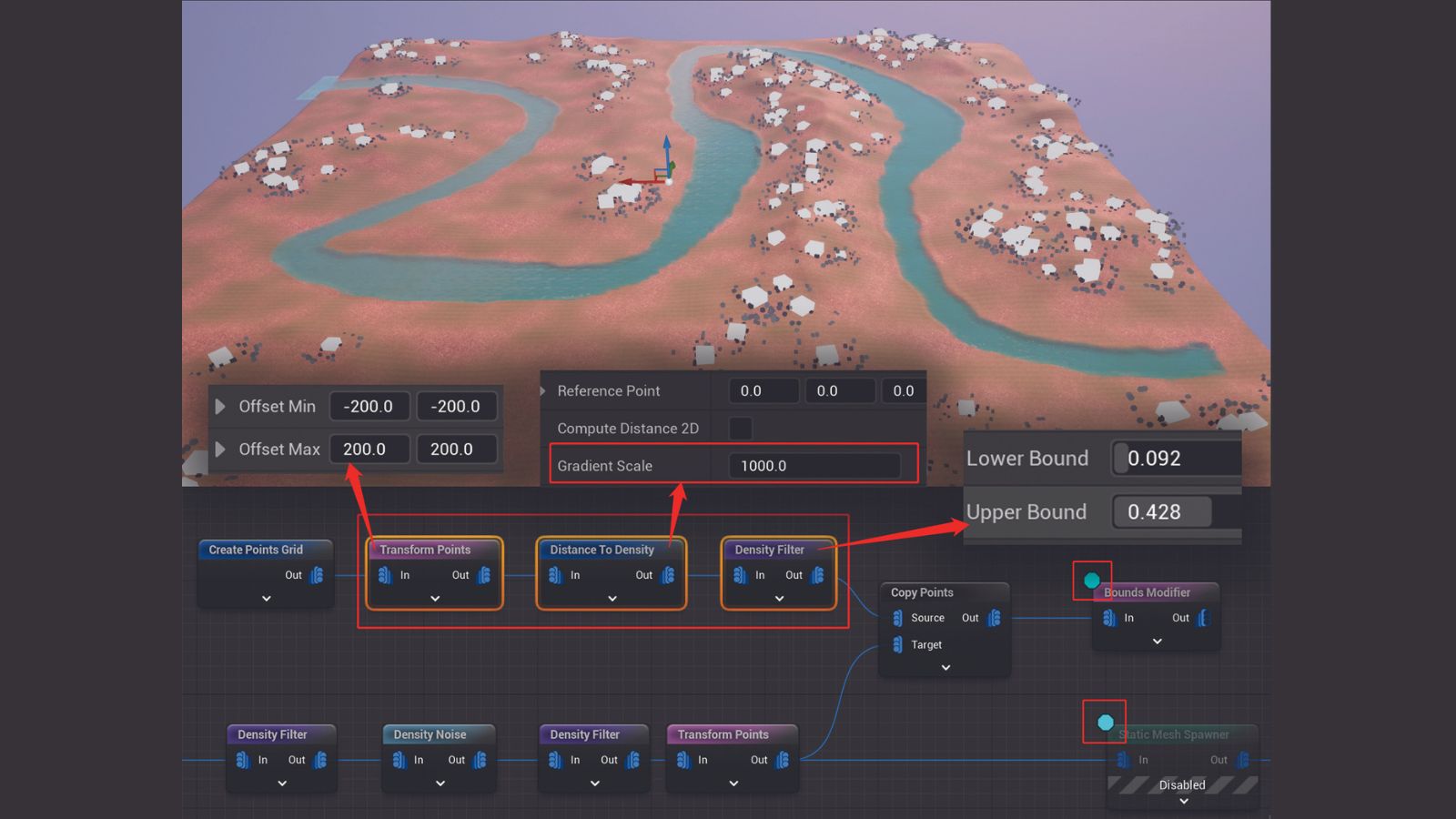
Insert Transform Points, Distance To Density, and Density Filter nodes between the Create Points Grid and Copy Points nodes. Set the Offset Min and Offset Max of the Transform Point node to -200, -200, 0 and 200, 200, 0 respectively to randomise the points’ positions.
Set the Gradient Scale of the Distance To Density node to 1000, which sets the density of each point based on their distance to the grid’s centre. For the Density Filter node, set the Lower and Upper Bounds to 0.092 and 0.428 to exclude any points that are too far from and too close to the centre. Enable debugging of the Static Mesh Spawner to see the new points.
12. Inserting grass around trees
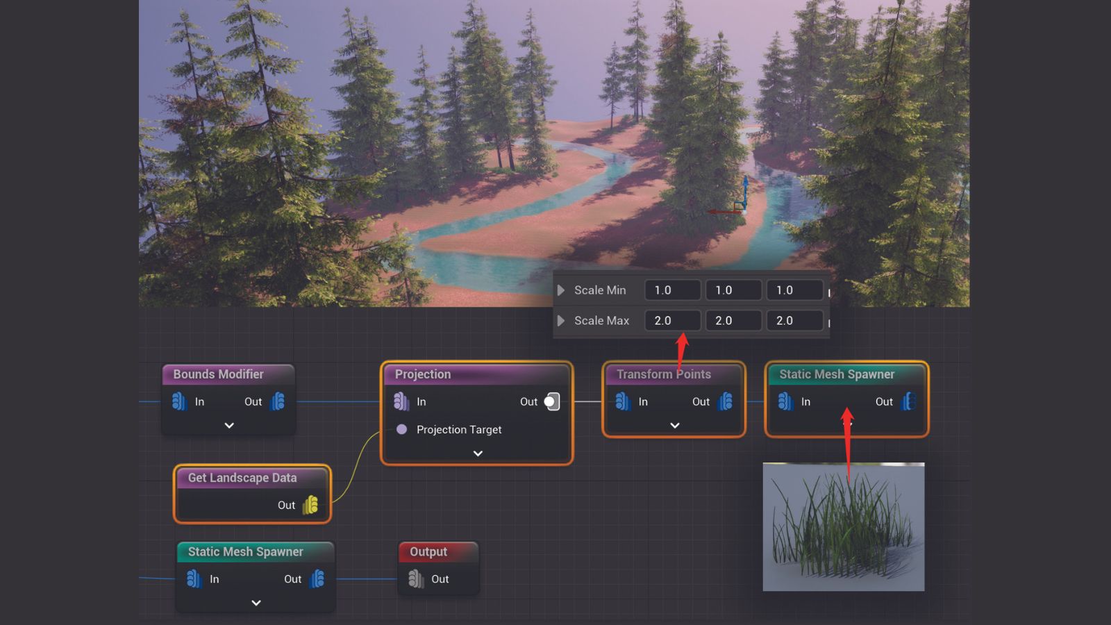
Add a Projection node after the Bound Modifier node and connect its Projection Target with a Get Landscape Data node. The Projection node projects the points to the surface of the Projection Target input, in this case onto the landscape’s surface.
Add a Transform Points node following the Projection node to add variation to the sizes of the points, and use another Static Mesh Spawner to instantiate grass. Enable the Static Mesh Spawner node of the trees to see both the trees and grass around their roots.
13. Refactor graph into subgraphs
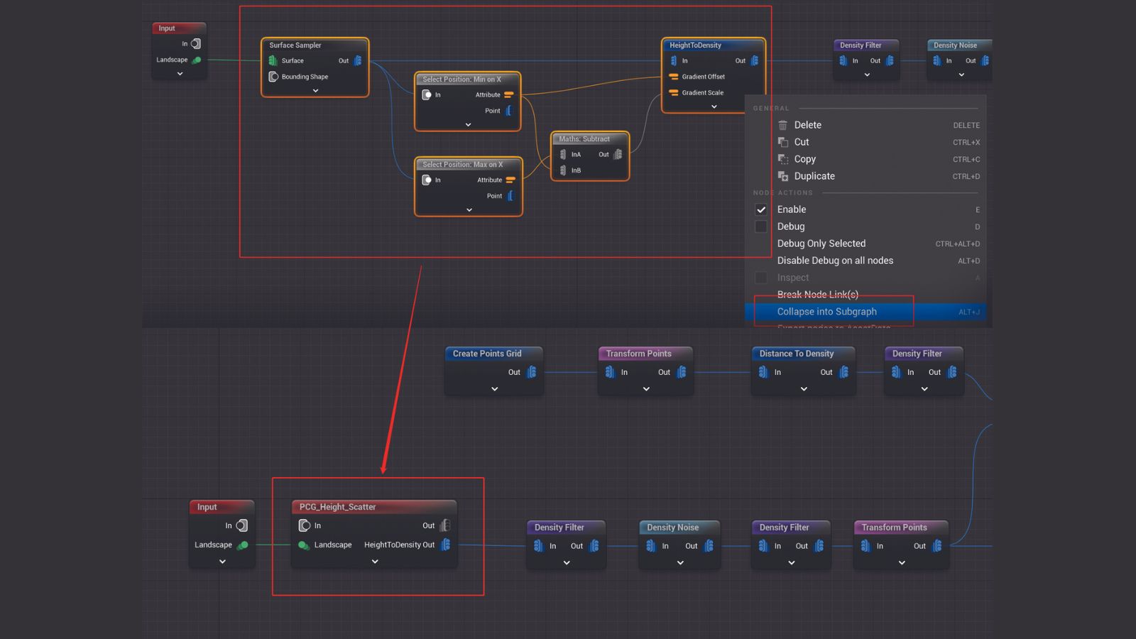
Select the nodes between and including the Surface Sampler and HeightToDensity nodes. Right-click any of them and click ‘Collapse into Subgraph’. Name the new subgraph ‘PCG_Height_Scatter’. The selected nodes now collapse into a single node, which is another PCG Graph, just like PCG_Forest. Open the new PCG_Height_Scatter node by double-clicking it, and you’ll see the chosen node now lives within.
14. Creating the scatter around subgraph
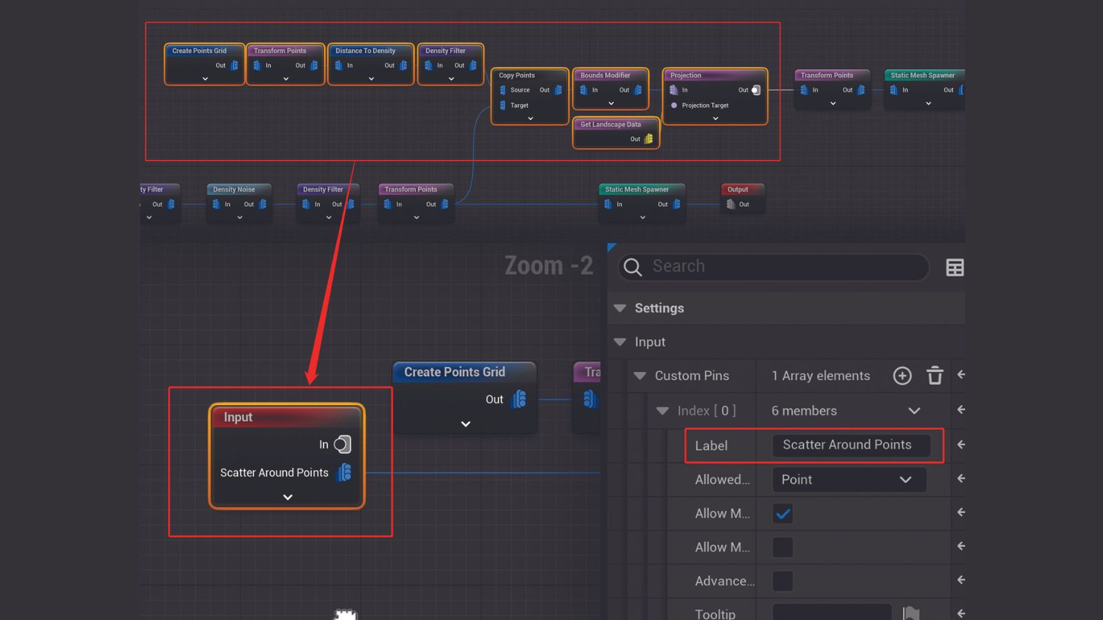
Select the nodes between and including the Create Points Grid and the Projection nodes, right-click, and make another subgraph named ‘PCG_Scatter_Around’. Doubleclick to open it, select the Input node, go to the Details panel and locate Input > Custom Pins > Index [0], and set its Label value to Scatter Around Points. This changes the input pin name to Scatter Around Points, which is more intuitive. The Custom Pins section lists all custom inputs of the subgraph. Adding extra inputs allows for fine-tuned control of the node’s behavior.
15. Adding more control to the subgraph
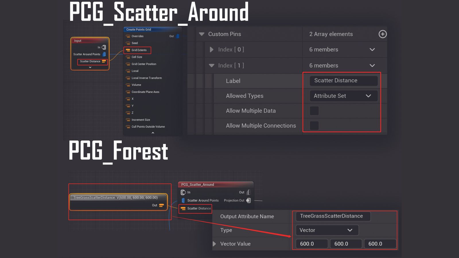
Select the Input node inside the PCG_Scatter_Around subgraph and add a new custom pin with ‘+’. Name the label Scatter Distance, change the Allowed Types to Attribute Set, and turn off Allow Multiple Data and Allow Multiple Connections. Connect the new Scatter Distance input to the Grid Extends input pin of the Create Points Grid node.
Go back to PCG_Forest and add a Create Attribute node, set its Output Attribute Name to TreeGrassScatterDistance, its Type to Vector, and its Vector Values to 600. Connect the Out pin of the node to the Scatter Distance input pin of PCG_Scatter_Around. The Create Attribute node now controls the scatter distance of the grass.
16. Creating realistic rocks
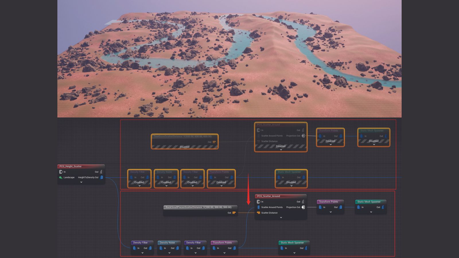
Select all the nodes after PCG_Height_Scatter, but don’t include the Output node. Press Ctrl+D to have a copy, and connect the HeightToDensity output of PCG_Height_Scatter to the newly duplicated Density Filter node. Disable the previously selected node and change the two duplicated Static Mesh Spawners to instantiate rocks.
Adjust the first Density Filter node to make the rocks appear between the water and trees. The Transform nodes are also adjusted so the rocks and small rocks around them are correctly sized. The new Create Attribute node is renamed RockSmallPiecesScatterDistance, and its values are also adjusted.
17. General foliage generation
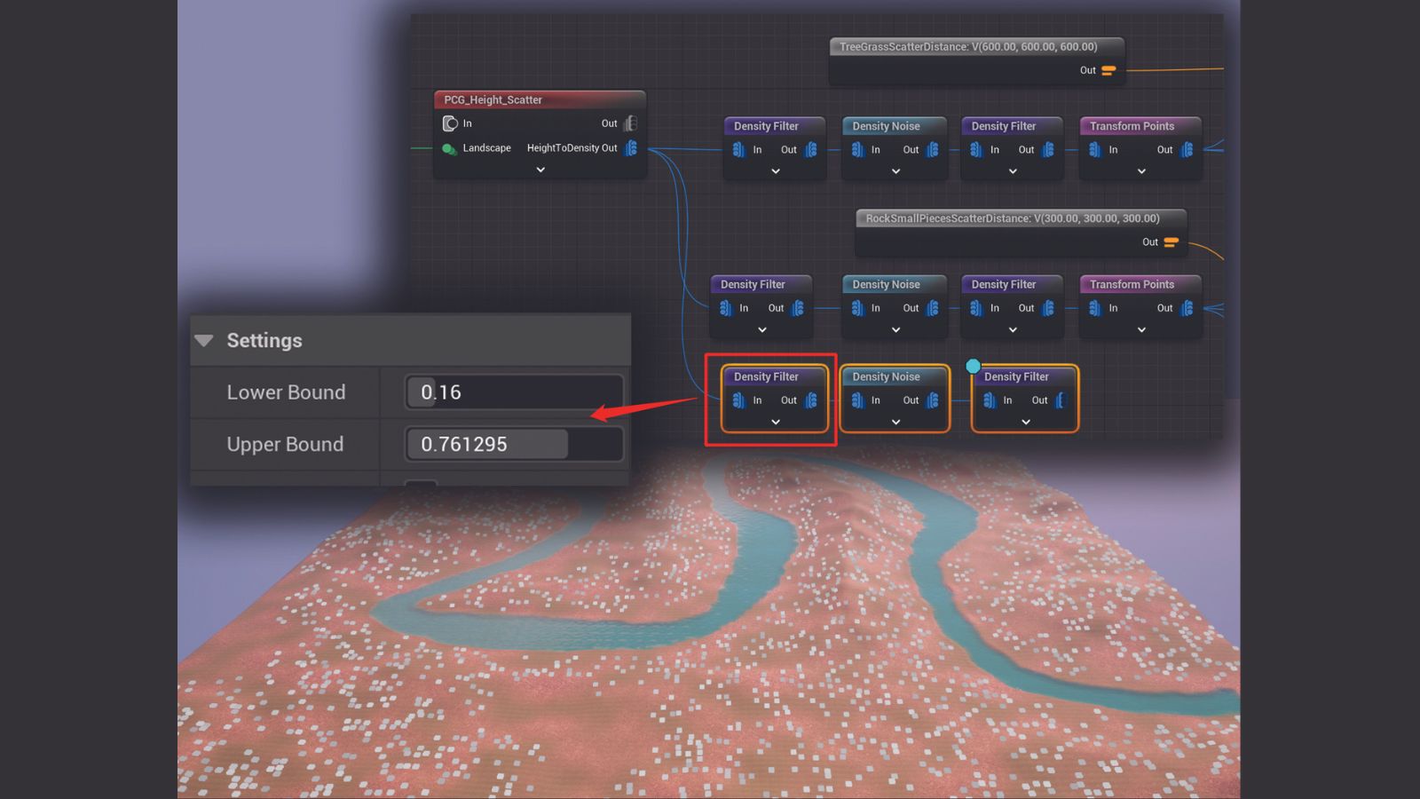
Enable everything but the Static Mesh Spawner nodes, duplicate the Density Filter, Density Noise, and Density Filter combo of the previous setup, and use it to scatter points on the landscape except the river. These will scatter random foliage. Be sure not to scatter too many points, as it may slow down the tool’s performance.
18. Excluding points blocked by assets
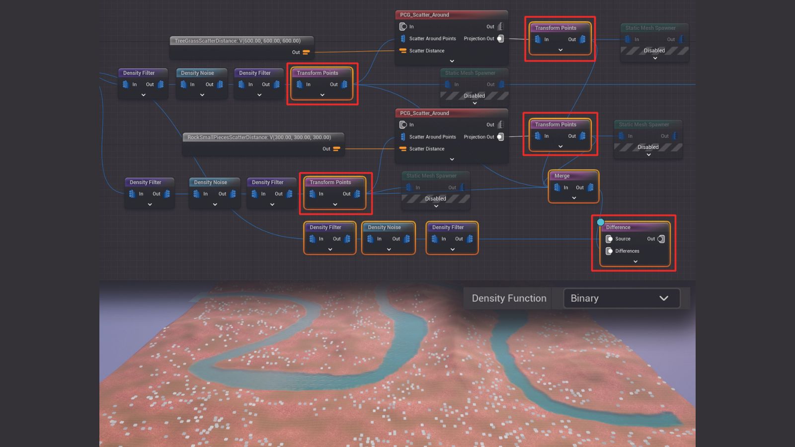
Create a Merge node and connect all four Transform Points nodes to it to merge the instantiation points of the trees and rocks together. Add a Difference node, connect the Merge node to its Difference input, and the last Density Filter created in the previous step to the Source input. Set the Density Function attribute of the Difference node to Binary. Enable debugging for the Difference node, and the points should only appear in areas that don’t have a tree or rock.
19. Adding more foliage
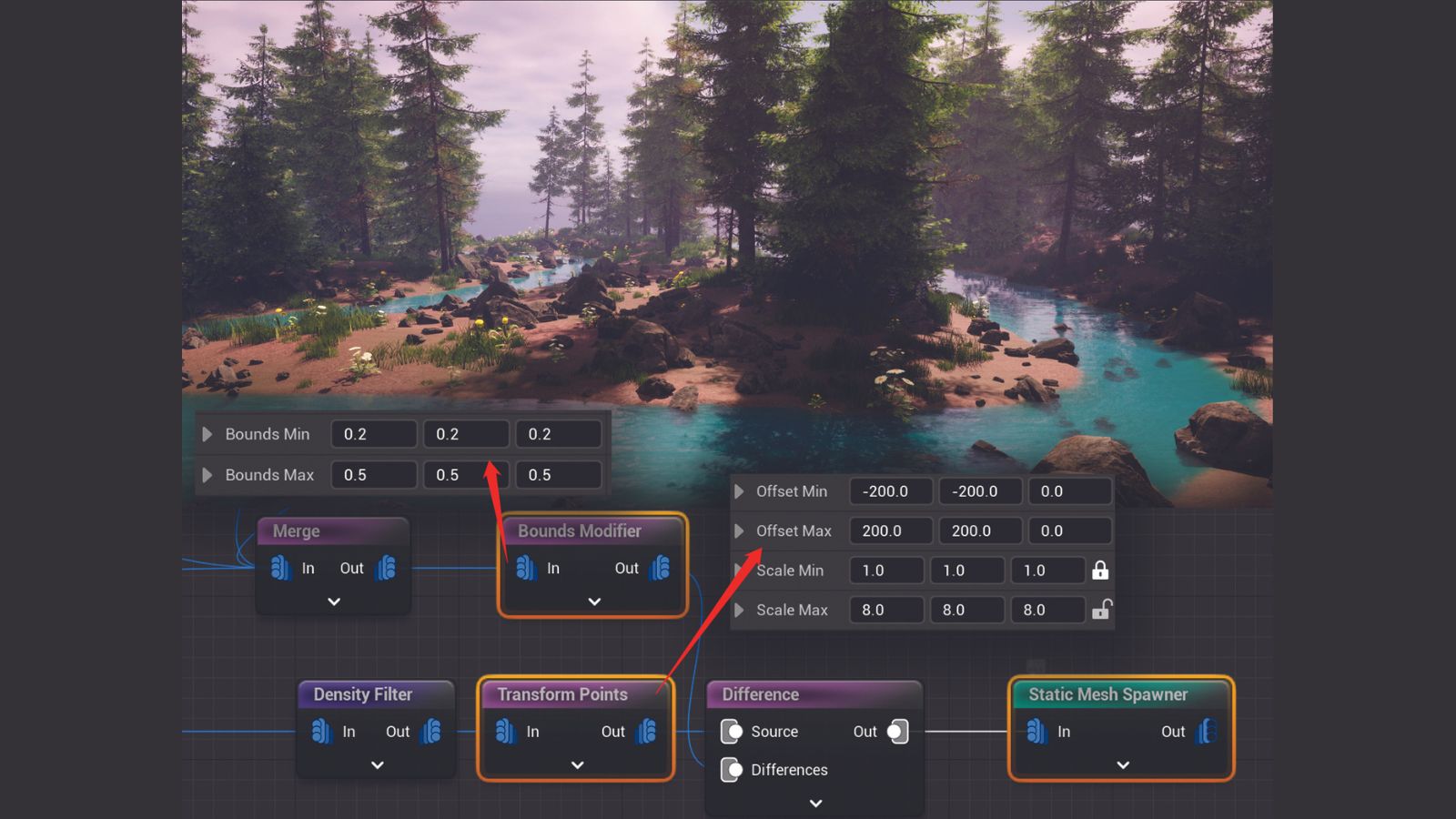
Create a Static Mesh Spawner after the Difference node and instantiate other foliage with it. Insert a Transform Points node between the Difference Node and the Density Filter node, and use it to randomly move and scale foliage. The values depend on the size and shape of the model provided in the Static Mesh Spawner node.
Add a Bounds Modifier node between the Merge and Difference nodes to shrink the bounds of the tree and rock points used to exclude foliage points. Enable all nodes, and adjust attributes for the desired look.
20. Sampling the river
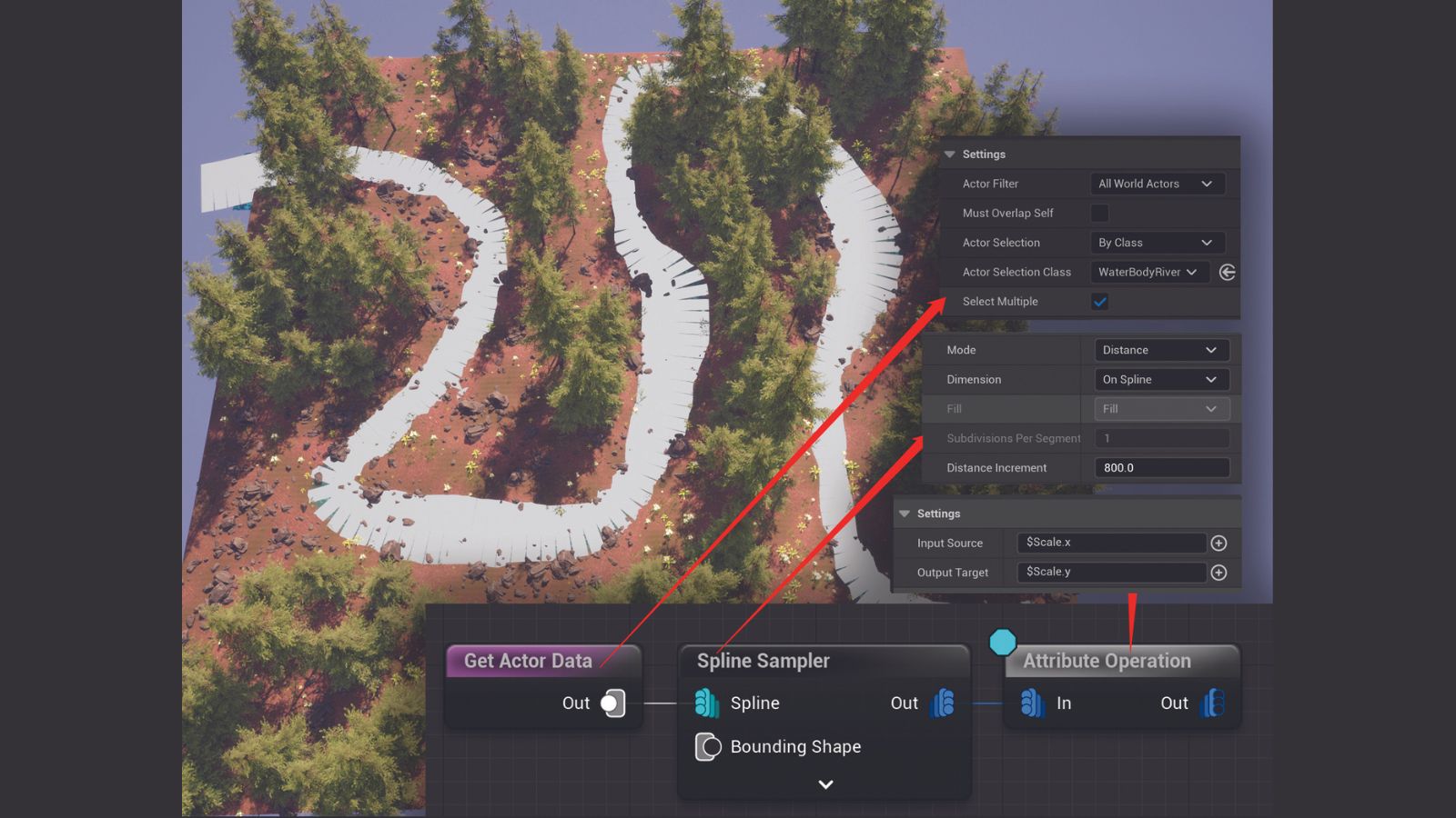
Create a Get Actor Data node, toggle on its Select Multiple, and set its Actor Filter to All World Actors, Actor Selection to By Class, and Actor Selection Class to WaterBodyRiver. It now collects all river actors as its output.
Create a Spline Sampler, and connect the Get Actor Data node to its Spline input, set its Mode to Distance, and Distance Increment to 800. River actors use the $Scale.x attribute of the spline points to determine the river’s width, but the spline sampler reads $Scale.y for the width of the points. To fix this, add an Attribute Operation node, set the Input Source to $Scale.x, and Output Target to $Scale.y.
21. Differentiate river points with distance
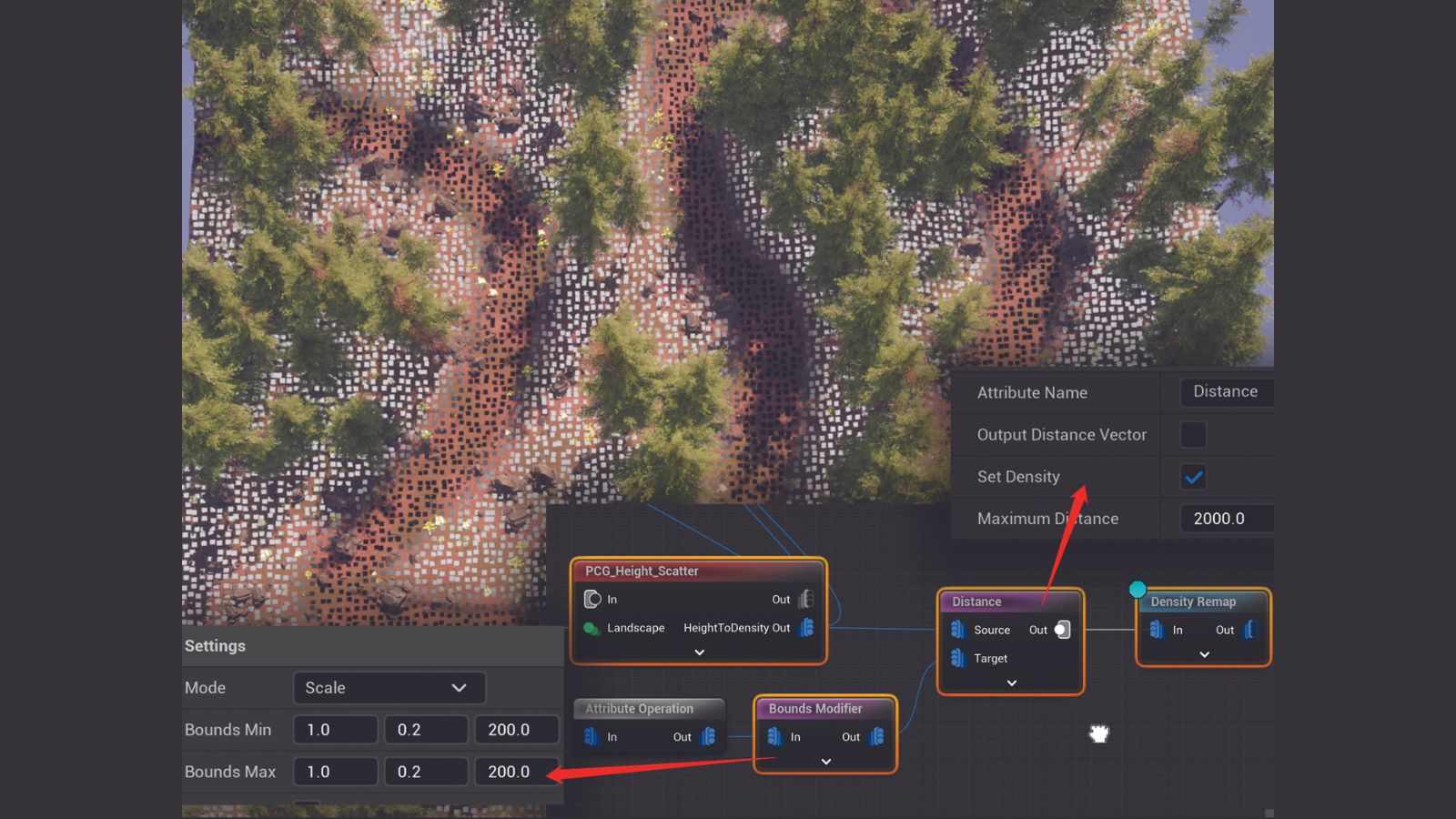
Add a Bound Modifier node after the Attribute Operation node, and set Bounds Min and Bounds Max to 1.0, 0.2, 200.0. Make a Distance node and connect PCG_Height_ Scatter’s second output to the Source input of the Distance node, connect the Bound Modifier to the Target input of the Distance node, check Set Density, and set the Maximum Distance to 2000. This node calculates the distance of points from PCG_Height_Scatter to the closest point of the Bounds Modifier and remaps their density.
Finally, Create a Density Remap node to clamp negative density values. Disable the visibility of the river to see the points under it.
22. Spawning river plants
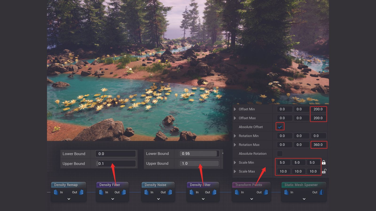
Create a Density Filter and set its Lower and Upper bounds to 0.0 and 0.1 to isolate points inside the river. Add a Density Noise and another Density Filter to filter out most of the points randomly.
Create Transform Points and Static Mesh Spawner nodes to instantiate aquatic plants. Notice the points are at the bottom of the river. To bring them up, a fixed offset is applied by checking the Absolute Offset of the Transform Points node, with the Offset Min and Max set to 200 on the Z axis.
23. Adding the riverbed's rocks
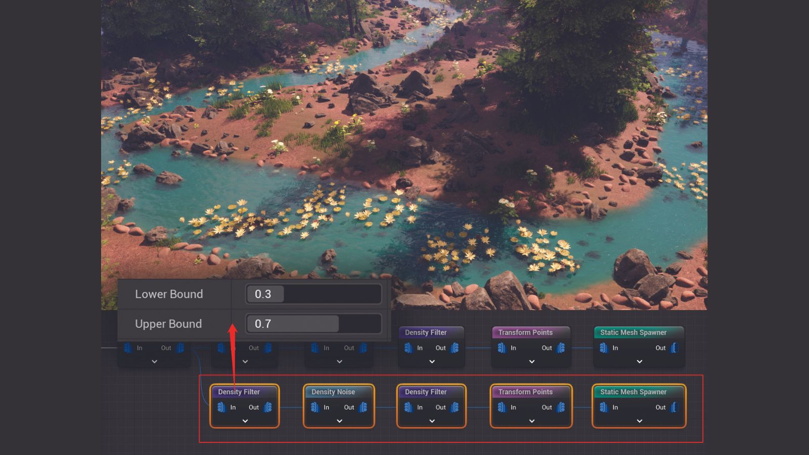
Using the above strategy, riverbed rocks are made on the edge of the river. The key change is different Lower and Upper Bound range at the first Density Filter to isolate points by the river.
Other tweaks could be made by repeating previous steps, such as to stop riverbed rocks overlapping with the foliage and rocks made previously. Use a Difference node to exclude the points that overlap.
24. PCG Blueprint Actor
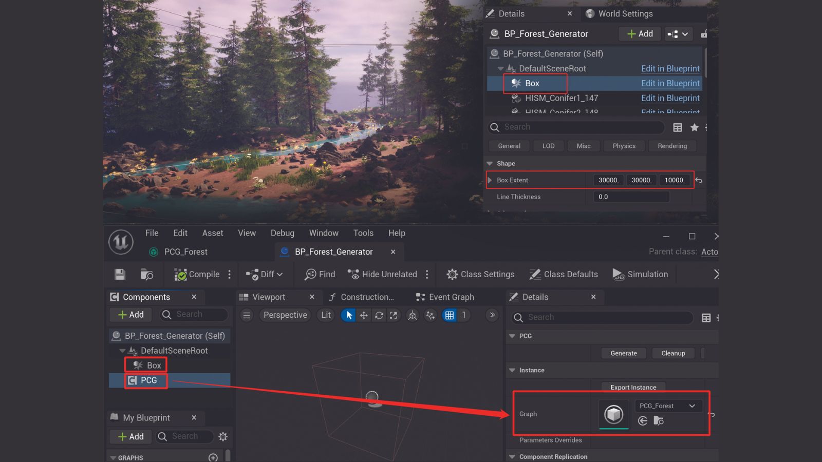
Create a Blueprint Actor, name it ‘BP_Forest_Generator’, open it, and add Box and PCG components. Select the latter and in the Details panel set the Graph attribute to PCG_Forest. Delete the PCG_Forest in the level and drag a BP_Forest_Generator in. The PCG component only creates meshes inside the actor’s bounding box, so to see its effect on the landscape, increase the Box Extent attribute of BP_Forest_Generator’s Box component to cover the area.
25. Using the Actor Seed control
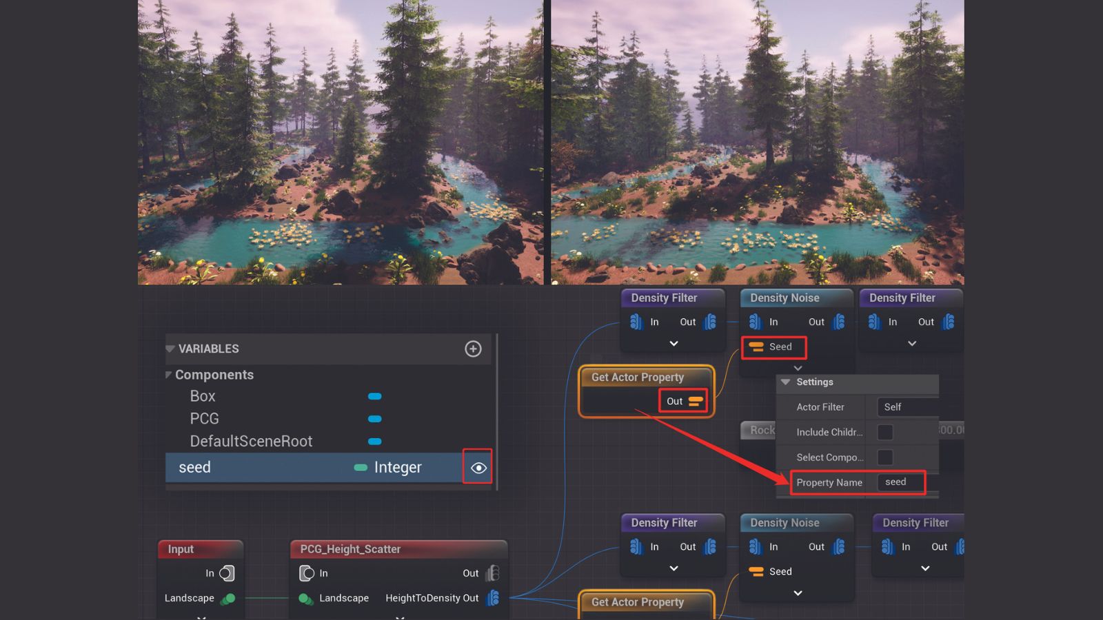
Add an integer variable named ‘Seed’ to BP_Forest_ Generator and expose it by clicking its eye icon. Go to PCG_Forest and create a Get Actor Property node, then set its Property Name to Seed to make it read the Seed variable value from its owning actor as its output. Connect the Actor Property node to the Seed input of all the Density Noise nodes. Back to the level, changing the Seed value of BP_Forest_Generator actor will yield a different variant of the forest.
26. Getting greater control
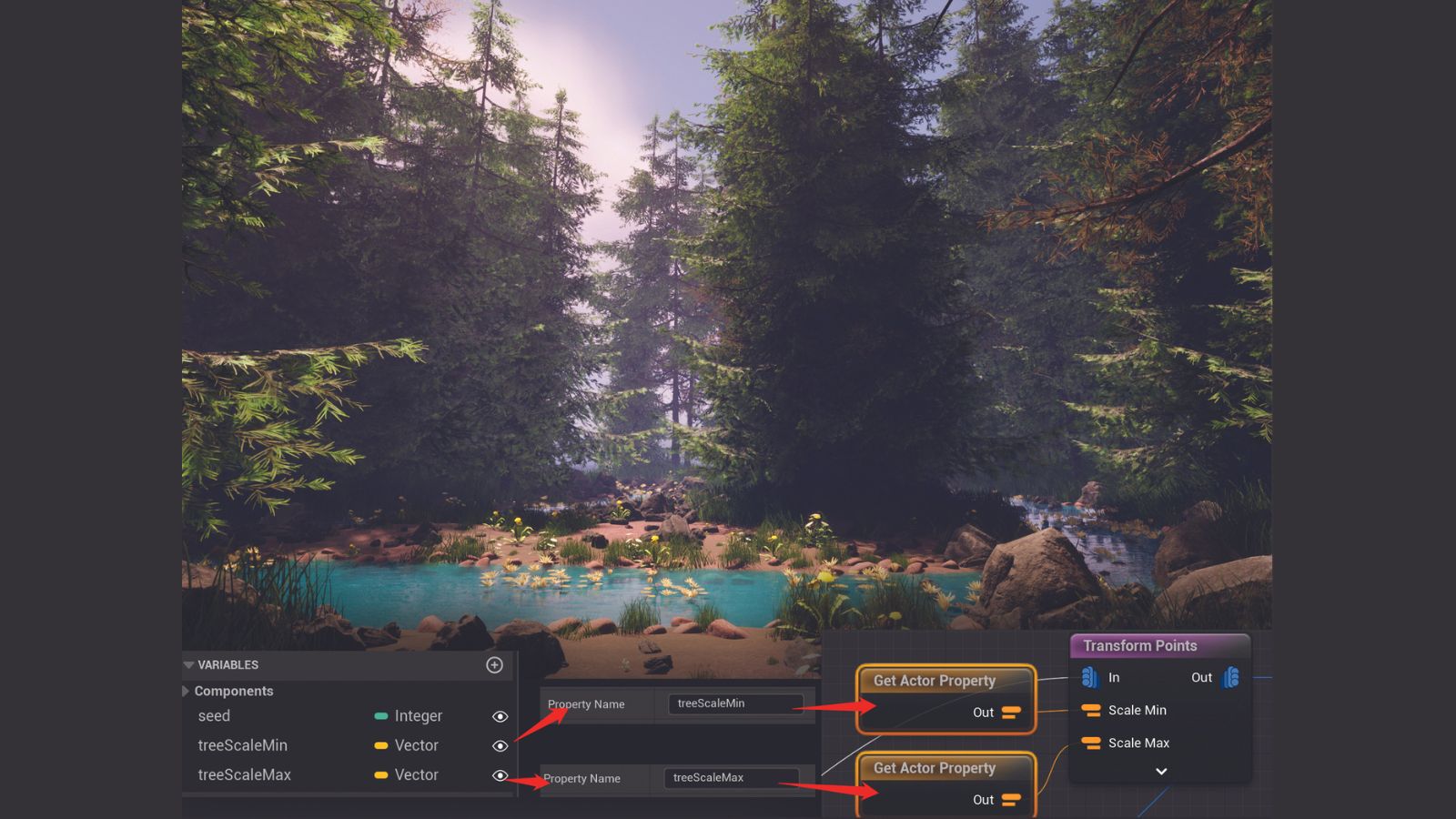
Add Vector variables to BP_Forest_Generator named ‘treeScaleMin’ and ‘treeScaleMax’, and expose both. In PCG_Forest, create two Get Actor Property nodes, one reading treeScaleMin and the other treeScaleMax. Connect these to the Scale Min and Scale Max attributes of the Transform Points node before the Static Mesh Spawner that makes the trees. The trees’ height can now be adjusted with the treeScaleMin and treeScaleMax variables of the BP_Forest_Generator actor. Repeat this method with more variables to gain even more control.
Making an environment in UE5: quick tips
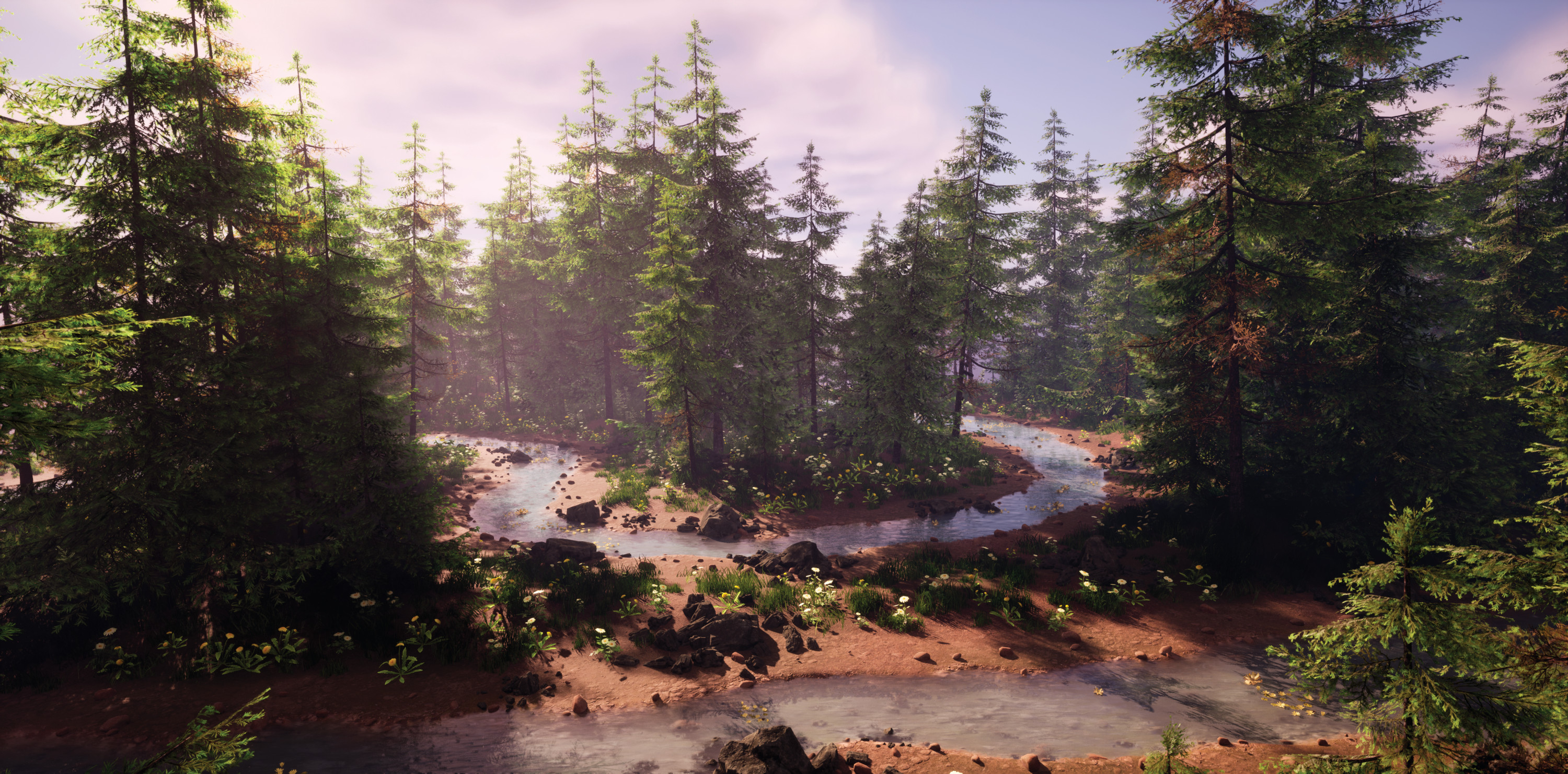
Here are a few more quick tips to keep in mind throughout this tutorial.
Adaptable graph
In step 4, we set the Gradient Scale of the HeightToDensity node to 2000, which remaps the density attribute from 0-1 for points with a height between 0-2000. But that means any points from 2000-4000 will have the same density value of 1. In step 5, we solved this by finding the lowest and highest Z positions and used that for the range. This guarantees the remap will be covered, no matter the landscape used as input.
Visualise what you're working on
In step 10, we disabled the Mesh Spawner to avoid blocking points we’ll be generating around it. It helps to isolate what you’re working on and disable the others. The Bounds Modifier helps us see the points more clearly; they might have been too small to see effectively before.
Bound modifier values
The bound width (extent) of the river points should be half the width of the river (bound extent is half the full size). However, we scale the Y (width) of the bounding box in the Bound Modifier to 0.2 instead of 0.5. This allows the slope of the riverbed to be within the spectrum of the density gradient generated by the Distance node. Adjust the values to see what effects it has.
Get more software tutorials in 3D World
This content originally appeared in 3D World magazine, the world's leading CG art magazine. 3D World is on sale in the UK, Europe, United States, Canada, Australia and more. Limited numbers of 3D World print editions are available for delivery from our online store (the shipping costs are included in all prices). Subscribe to 3D World at Magazines Direct.
