
Ever find yourself with a Microsoft Excel spreadsheet jam-packed full of data but don't know where to look next? Do you wish you could sift, sort, and analyze and make your data work harder for you? Well, look no further. With this guide, we'll look at 7 handy tools to make your data much more accessible, giving you the top-line information you need (and looking good while doing so!).
The following Excel functions can be used on new or existing databases to find or summarise information quickly and easily. You can use them to turn a wall of numbers into meaningful data with just a few simple clicks.
Although we have only provided 7 tools here, they will make a huge difference to your capabilities. You can even combine most of them to enhance their impact even further, leaving your boss and colleagues in awe of your skills.
Most of these tools are relatively basic, but a few of the later ones may border on intermediate. Although, with a bit of practice, anyone can use them successfully and give your Microsoft Office projects that wow factor.
So without further ado, let's look at our first simple tool to get your data working.
Sum
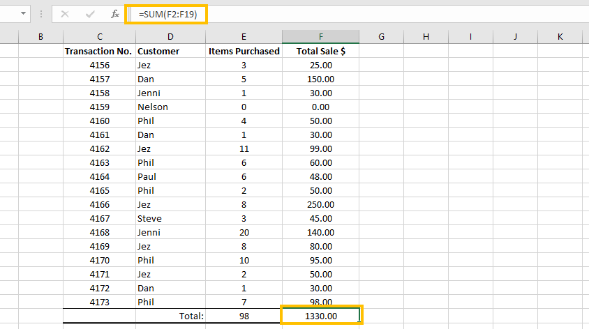
It’s as simple as it sounds. Use the Sum function to Sum (add up) all of the requested data. You can do this across rows or columns, even adding together multiple numerical sources on your spreadsheet.
Let's have a look at creating a basic Sum formula:
=Sum(value1,value2,value3…)To sum a range of data, you replace the value in the formula with the cells. For example, to add cells A1 through to A20, you would use ”Sum(A1:A20)”. Further cells or ranges can be added following a comma “=Sum(A1:A20, B15, C2:C5)”.
You can instruct the formula exactly which cells to include by typing in the cell names, or you can click and drag a box over the cells you wish to include, and the formula will automatically add these.
You can choose to Sum at the end of a row or column or make a table elsewhere on your sheet. You can even Sum the contents of one sheet and have them pull through the results to another sheet (or even workbook) entirely. Still a simple tool, but much more functional than it first appears.
Count
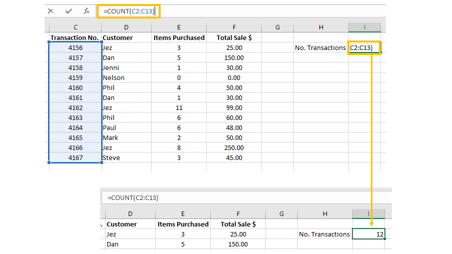
The most basic Count function does exactly what it says. It counts the total number of cells highlighted in a range. It does not, however, add up the total of the contents in the cells, just the number of cells present. We use the following formula:
=Count(value1,value2,value3…)Inside the brackets, you can either list the individual values/cells or put in the range of cells you wish to consider. A range can be across multiple rows and columns, like A1:A50 or A1:D50.
The above example shows the total number of transactions made by customers in a small database.
The Count function will only count cells that contain numbers, so if a cell is blank or contains text, it will ignore the cell completely.
If you would like to count cells in a more specific manner, such as cells that contain a certain number or a certain string of text, then read on for the more powerful CountIf!
CountIf
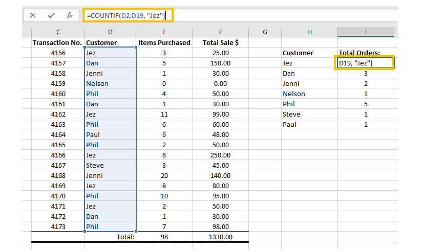
This function will only count cells if they meet specified criteria (really living up to its name!). For example, you may want to only count cells containing a certain name or ID number or a value above or below a certain threshold.
=CountIf(range,criteria)We select a range similar to the previous count function, then place a comma and state the criteria you wish to consider. In the below example, I added a count of the number of orders for each customer by counting how many times their name appears on the order list in the above example.
If we wanted to, say, count sales only above $100, you would simply set the criteria in the formula as >100. To do this, the formula would be “=CountIf(F1:F19, “>100”)”. The criteria can be quite versatile; you can count by numbers in a range, count if it’s a specific piece of text, or count if it matches the content of another specified cell.
SumIf
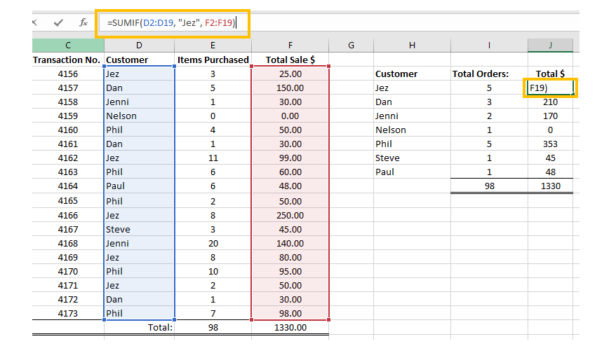
Similar to CountIf, we can use SumIf to only consider the cells which meet our given set of criteria. The difference here is, Countif will only count the number of cells, whereas SumIf will sum the contents of the cells if they match your set of guidelines.
=SumIf(range,criteria,[sum_range])You can build up a whole string of different criteria, just like CountIf does above, to sum data in multiple cells which meet your strict set of rules. One difference you will notice is the inclusion of [sum_range] in the formula. This lets us specify the rules in one column but add the values from another corresponding column.
Building on the previous example, you can see here that I used SumIf to create a table to add up the order value for each customer, using their name as the criteria. On the spreadsheet extract (see above), the cells highlighted in blue are the cells it checks for criteria; then, if it’s a match, the cells in red are summed up.
Min / Max
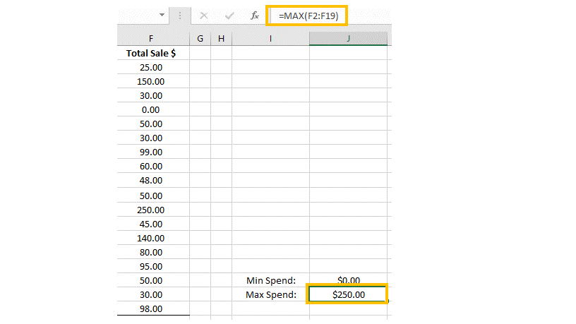
This nifty function will simply pull out the highest or lowest values from a set of numbers to save you from having to trawl through lines and lines of info, playing spot the difference. This can be useful for seeing at a glance which customer is spending the most money with your business or, for example, if you have a list of times of marathon runners, it can instantly show you the fastest or slowest times achieved.
=Min(value1,value2,value3…)
or
=Max(value1,value2,value3…)This little tool can be a real time saver. As your data changes the ranks, the Min and Max will always stay up to date by constantly looking at the formula and making sure it's correct.
You can combine this with some conditional formatting to make the cells or text a different style of color or pull the information through to an overview page to always ensure you are up to date with any changes.
Rank
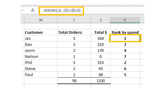
Rather than just seeing the highest and lowest values with the Min/Max functions, you can also rank a selection of data by their individual values. This is done using the rank formula.
Depending on what data you have, the Rank function can be used to quickly view where you need to focus your attention, such as which products are making the least sales or which webpages are receiving the highest clicks.
Let's look at an example:
=RANK(number,ref,[order])You select the number to which you wish to assign a rank, then the ‘ref’ is the group of values it is being compared to, followed by the optional ‘order’ value – this can be either 0 for descending or 1 for ascending.
Our above example shows which of our customers are making the most / least expenditure on sales. We could easily change to look at the volume of sales instead by selecting the previous column, depending on our needs at the time.
Again, you can even pair this with some conditional formatting to make the highest and lowest ranks stand out or even put each rank on a sliding color scale to really give it some flair.
Vlookup
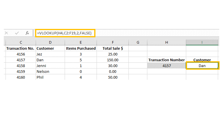
The infamous VLookup is extremely useful but not nearly as difficult as its reputation suggests. By entering a unique value from the first column of your table (such as an order number, ID number, or name), the Vlookup function will scour the entire table and bring back some specific data related to your input.
Using our customer database from above, we can type the unique transaction number from the first column to pull up all details related to that transaction.
The formula used for this is:
=VLOOKUP(lookup_value,table_array,col_index_num,[range_lookup)Although this looks complicated at first, it's actually quite straightforward. Let's break it down:
Lookup_value is the cell it reads before it goes off searching. This is a unique string of information you type to prompt the search. For example, you might type in a transaction number to look up a specific customer sale.
Table_array is the search location. Here you specify what data you want to be included in the search, and the function will search this table each time you enter a lookup value. Your unique lookup_value should always be in the first column in this table.
Col_index_num is the column from the above Table_array, which will provide you with the data to output. The lookup will take your lookup_value, find it in the table_array and then provide the data which is present in the column number we have entered here.
Range_lookup is an optional field. Here you can enter either TRUE or FALSE. If TRUE, then the lookup will search for an approximate match. If FALSE, then the lookup wants an exact match. If left blank, this will always default to TRUE.
In the example, the VLOOKUP formula in cell I4 reads the transaction number from cell H4. It finds this number in the table, then looks at column 2, which in this case is the customer name. It then reads across to this column and sends back the name Dan.
By extending the Vlookup to more additional cells, we can create a full recount of the customer order made with each transaction number. You only need to change the column number to look at the adjacent information to pull that through too.
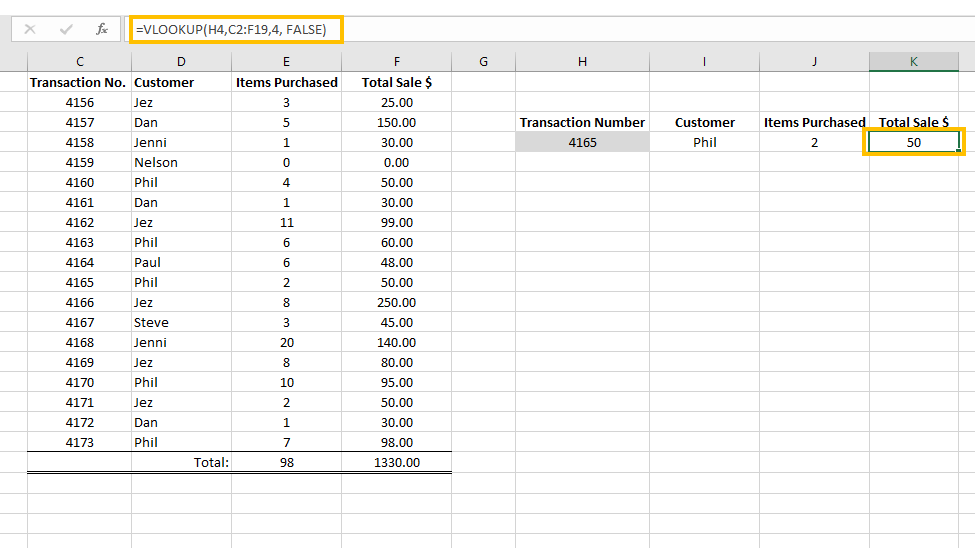
As useful as they are, Vlookups do come with a couple of limitations. Firstly, the VLookup value will not recognize any duplicate values. If we had two transactions with the same ID number, the function would find the first occurrence and then stop. This is why it is important to have a unique value – If we used surnames, for example, and had 2 Smiths, the Vlookup would always stop at the first Smith.
Secondly, Vlookups can only look right. This isn't a Zoolander reference but a feature of how the search works. It looks down the left-hand column for the 'Lookup_value' and then returns information from the columns to the right of this (as specified by the user). There are way around this, such as the XLOOKUP function, but they are a bit more advanced.
By implementing and combining all of the Excel devices we have discussed, your spreadsheet will be constantly crunching numbers in the background while you put your feet up or grab another coffee. Collate everything into a simple dashboard or front page, and your data can look like a bespoke software package designed by and for you.
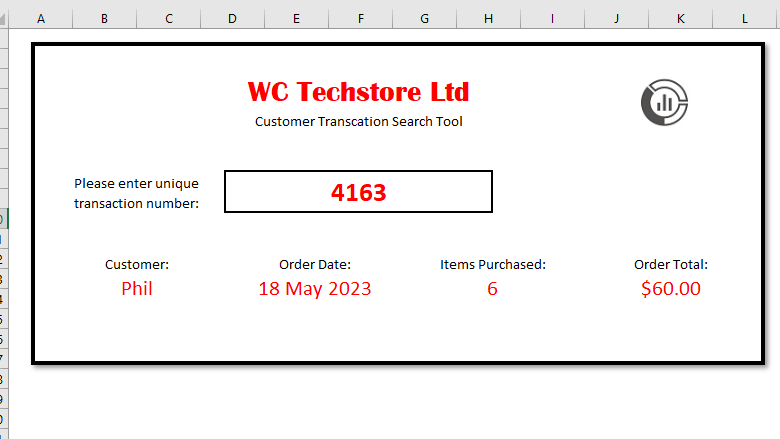
Using the tools in this article, along with the tips featured in our 10 top Microsoft Excel tips to help you become a spreadsheet sorcerer, you will be creating complex databases in no time. Add a little bit of your own style and flair, and you can easily create professional-looking pages to wow your colleagues and customers or even just impress yourself.
By putting in a little bit of time and effort during the creation of your spreadsheet, you can prolong its life and usability, making it work for you. Your data can keep you informed and save precious hours, all whilst looking good at the same time.
More resources
For more helpful articles, coverage, and answers to common questions about Windows 10 and Windows 11, visit the following resources:


